- Quick description
- General discussion
- Prerequisites
- Example 1: convexity of norms
- Example 2: the maximum principle
- Example 3: new Strichartz estimates from old
- Example 4: the Hausdorff-Young inequality
- Example 5: an example from additive combinatorics, due to Imre Ruzsa
- Example 6: the Cotlar-Knapp-Stein lemma
- Example 7: entropy estimates
- Example 8: the monotonicity of Perelman's reduced volume
- Example 9: the Riemann hypothesis for function fields
- Further reading
Quick description
If one wants to prove an inequality  for some non-negative quantities
  ,
,  , but can only see how to prove a quasi-inequality
  that loses a multiplicative constant
  , then try to replace all objects involved in the problem by "tensor powers" of themselves and apply the quasi-inequality to those powers. If all goes well, one can show that
  for all
  , with a constant which is independent of
  , which implies that as desired by taking
  roots and then taking limits as
  .
.
General discussion
This trick works best when using techniques which are "dimension-independent" (or depend only weakly (e.g. polynomially) on the ambient dimension ). On the other hand, the constant is allowed to depend on other parameters than the dimension . In particular, even if the eventual inequality one wishes to prove is supposed to be uniform over all choices of some auxiliary parameter n, it is possible to establish this estimate by first establishing a non-uniform estimate  , so long as this estimate "tensorises" to
  , where
  does not grow with .
It is of course essential that the problem "commutes" or otherwise "plays well" with the tensor power operation in order for the trick to be effective. In order for this to occur, one often has to phrase the problem in a sufficiently abstract setting, for instance generalizing a one-dimensional problem to one in arbitrary dimensions.
Prerequisites
Advanced undergraduate analysis (real, complex, and Fourier). The user of the trick also has to be very comfortable with working in high-dimensional spaces such as  , or more generally
  for some mathematical object
  (e.g. a set, a group, a measure space, etc.) The later examples are more advanced but are only given as sketches.
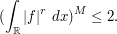
Example 1: convexity of  norms
norms
Let  be a measurable function such that
  and
and  for some
  . Show that
  for all
  .
.
As a first attempt to solve this problem, observe that  is less than
  when
when  , and is less than
  when
when  . Thus the inequality
  holds for all x, regardless of whether
  is larger or smaller than 1. This gives us the bound
  , which is off by a factor of 2 from what we need.
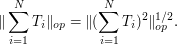
But we can eliminate this loss of 2 by the tensor power trick. We pick a large integer  , and define the tensor power
 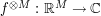 of f by the formula

From the Fubini–Tonelli theorem we see that
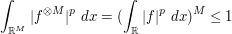
and similarly
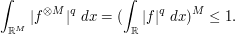
If we thus apply our previous arguments with  and
and  replaced by
  and respectively, we conclude that
applying Fubini–Tonelli again we conclude that
Taking roots and then taking limits as we
obtain the claim.
Exercise
More generally, show that if 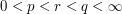 ,
,  is a measure space, and
  is measurable, then we have the inequality

whenever the right-hand side is finite, where  is such that
 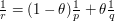 . (Hint: by multiplying f and
  by appropriate constants one can normalize
  .)
.)
Exercise
Use the previous exercise (and a clever choice of f, r,  and - there is more than one choice available) to prove Hölder's inequality.
Example 2: the maximum principle
This example is due to Landau. Let  be a simple closed curve in the complex plane that bounds a domain D, and let
  be a function which is complex analytic in the closure of this domain, and which obeys a bound
  on the boundary . The maximum principle for such functions asserts that one also has
  on the interior
  as well. One way to prove this is by using the Cauchy integral formula
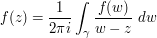
for  (assuming that is oriented anti-clockwise). Taking absolute values and using the triangle inequality, we obtain the crude bound
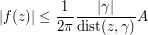
where  is the length of . This bound is off by a factor of
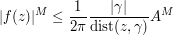
  . This loss depends on the point z and the curve , but it is crucial to observe that it does not depend on f. In particular, one can apply it with f replaced by
  (and A replaced by
  ) for any positive integer , noting that is of course also complex analytic. We conclude that
and on taking roots and then taking limits as
we obtain the maximum principle.
Example 3: new Strichartz estimates from old
This observation is due to Jon Bennet. Technically, it is not an application of the tensor power trick as we will not let the dimension go off to infinity, but it is certainly in a similar spirit.
Strichartz estimates are an important tool in the theory of linear and nonlinear dispersive equations. Here is a typical such estimate: if 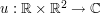 solves the two-dimensional Schrödinger equation
  , then one has the inequality

for some absolute constant . (In this case, the best value of is known to equal  , a result of Foschi and of Hundertmark-Zharnitsky.) It is possible to use this two-dimensional Strichartz estimate and a version of the tensor power trick to deduce a one-dimensional Strichartz estimate. Specifically, if
  solves the one-dimensional Schrödinger equation
  , then observe that the tensor square
  solves the two-dimensional Schrödinger equation. (This tensor product symmetry of the Schrödinger equation is fundamental in quantum
physics; it allows one to model many-particle systems and single-particle systems by essentially the same equation.) Applying the above Strichartz inequality to this product we conclude that
solves the two-dimensional Schrödinger equation. (This tensor product symmetry of the Schrödinger equation is fundamental in quantum
physics; it allows one to model many-particle systems and single-particle systems by essentially the same equation.) Applying the above Strichartz inequality to this product we conclude that

Remark
A similar trick allows us to deduce "interaction" or "many-particle" Morawetz estimates for the Schrödinger equation from their more traditional "single-particle" counterparts; see for instance Chapter 3.5 of Terence Tao's book.
Example 4: the Hausdorff-Young inequality
Let be a finite abelian group, and let 
 be the group of characters
  of G, and define the Fourier transform
  by the formula
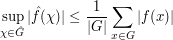
From the triangle inequality we have
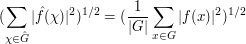
while from Plancherel's theorem we have
By applying the Riesz-Thorin interpolation theorem, we can then conclude the Hausdorff-Young inequality
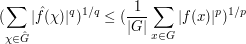
whenever  and
and  . However, it is also possible to deduce (3) from (2) and (1) by a more elementary method based on the tensor power trick. First suppose that is supported on a set
  and that
  takes values between (say)
  and
and  on
on  . Then from (1) and (2) we have
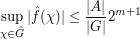
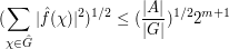
from which we establish a "restricted weak-type" version of Hausdorff-Young, namely
and thus
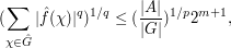
This inequality is restricted to those whose non-zero magnitudes range inside a dyadic interval ![{}[2^m, 2^{m+1}]](../images/tex/a6011a5d0044be110b1a2a8be0faa7f7.png) , but by the technique of dyadic decomposition one can remove this restriction at the cost of an additional factor of
, but by the technique of dyadic decomposition one can remove this restriction at the cost of an additional factor of  , thus obtaining the estimate
for general . (There are of course an infinite number of dyadic scales in the world, but if one normalizes 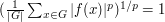 , then it is not hard to see that any scale above, say,
  or below
  is very easy to deal with, leaving only
  dyadic scales to consider.)
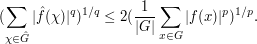
The estimate (4) is off by a factor of from the true Hausdorff-Young inequality, but if one replaces G with a Cartesian power and f with its tensor power , and makes the crucial observation that the Fourier transform of a tensor power is the tensor power of the Fourier transform, we see from applying (4) to the tensor power that
dyadic scales to consider.)
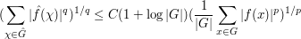
The estimate (4) is off by a factor of from the true Hausdorff-Young inequality, but if one replaces G with a Cartesian power and f with its tensor power , and makes the crucial observation that the Fourier transform of a tensor power is the tensor power of the Fourier transform, we see from applying (4) to the tensor power that
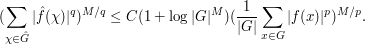
Taking roots and sending we obtain the desired inequality. Note that the logarithmic dependence on  in the constants turned out not to be a problem, because
  . Thus the tensor power trick is able to
handle a certain amount of dependence on the dimension in the constants, as long as the loss does not grow too rapidly in that dimension.
. Thus the tensor power trick is able to
handle a certain amount of dependence on the dimension in the constants, as long as the loss does not grow too rapidly in that dimension.
Exercise
Establish Young's inequality  for
for  and
and  and finite abelian groups , where
  , by the same
method.
, by the same
method.
Exercise
Prove the Riesz-Thorin interpolation theorem by this method, thus avoiding all use of complex analysis. (Note the similarity here with Example 1 and Example 2.)
Example 5: an example from additive combinatorics, due to Imre Ruzsa
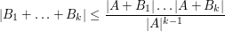
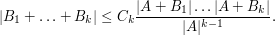
An important inequality of Plünnecke asserts, among other things, that for finite non-empty sets ,  of an additive group , and any positive integer
  , the iterated sumset
  , which is defined as the set of all possible sums of not necessarily distinct elements of , obeys the bound
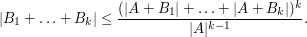
(This inequality, incidentally, is itself proved using a version of the tensor power trick, in conjunction with Hall's marriage theorem, but never mind that here.) This inequality can be amplified to the more general inequality
via the tensor power trick as follows. Applying (5) with  , we obtain
The right-hand side looks a bit too big, but we can resolve this problem with a Cartesian product trick (which can be viewed as a cousin of the tensor product trick). If we replace with the larger group  and replace each set
  with the larger set
 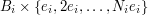 , where
  is the standard basis for
  and
and  are arbitrary positive integers (and replacing with
  ), we obtain

Optimizing this in  (basically, by making the
  close to constant; this is a general rule in
optimization, namely that to optimize
close to constant; this is a general rule in
optimization, namely that to optimize  it makes sense to make and comparable in magnitude – someone should think of some examples and write a Tricki article on this) we obtain the amplified estimate
for some constant  ; but then if one replaces
  with their Cartesian powers
  roots, and then sends to infinity, one can delete the constant and recover the inequality.
Example 6: the Cotlar-Knapp-Stein lemma
This example is not exactly a use of the tensor power trick, but is very much in the same spirit. Let  be bounded linear operators on a Hilbert space; for simplicity of discussion let us say that they are self-adjoint, though one can certainly generalize the discussion here to more general operators. If we assume that the operators are uniformly bounded in the operator norm, say

for all  and some fixed , then this is not enough to ensure that the sum
  is bounded uniformly in
  ; indeed, the operator norm can be as large as
  . If however one has the stronger almost orthogonality estimate
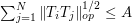
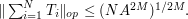
for all , then the very useful Cotlar-Knapp-Stein lemma asserts that is now bounded uniformly in , with 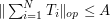 . To prove this, we first recall that a direct application of the triangle inequality using (6) (which is a consequence of (7)) only gave the inferior bound of . To improve this, first observe from self-adjointness that
Expanding the right-hand side out using the triangle inequality, we obtain

using (7) one soon ends up with a bound of  is concerned, but one can do better by using higher powers. In particular, if we raise
  to the
  power for some M, and repeat the previous arguments, we end up with

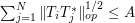
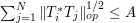
Now, one can estimate the operator norm  either by

or (using (6)) by

We take the geometric mean of these upper bounds to obtain

Summing this in  , then
  , and so forth down to
  using (7) repeatedly, one eventually establishes the bound
Sending one eliminates the dependence on and obtains the claim.
Exercise
Show that the hypothesis of self-adjointness can be dropped if one replaces (7) with the two conditions
and
for all .
Example 7: entropy estimates
Suppose that is a random variable taking finitely many values. The Shannon entropy  of this random variable is defined by the formula
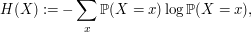
where  runs over all possible values of . For instance, if is
uniformly distributed over values, then
runs over all possible values of . For instance, if is
uniformly distributed over values, then

If is not uniformly distributed, then the formula is not quite as simple. However, the entropy formula (8) does simplify to the uniform distribution formula (9) after using the tensor power trick. More precisely, let  be the random variable formed by taking M independent and identicaly distributed samples of ; thus for instance, if was uniformly distributed on values, then
  is uniformly distributed on
  values. For more general , it is not hard to verify the formula
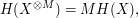
which is of course consistent with the uniformly distributed case thanks to (9).
A key observation is that as , the probability distribution of becomes "asymptotically uniform" in a certain sense. Indeed, the law of large numbers tells us that with very high probability, each possible value of will be attained by 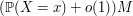 of the trials
  . The number of possible configurations of which are consistent with this distribution can be computed (using Stirling's formula) to be
  , and each such configuration appears with probability
  (again by Stirling's formula). Thus, at a heuristic level at least, behaves like a uniform distribution on possible values; note that this is consistent with (9) and (10), and can in fact be taken as a definition of Shannon entropy.
One can use this "microstate" or "statistical mechanics" interpretation of entropy in conjunction with the tensor power trick to give short (heuristic) proofs of various fundamental entropy inequalities, such as the subadditivity inequality

whenever , are discrete random variables which are not necessarily independent. Indeed, since and  (heuristically) take only and
  values respectively, then
  will (mostly) take on at most
  values. On the other hand, this random variable is supposed to behave like a uniformly distributed random variable over
  values. These facts are only compatible if

taking roots and then sending we obtain the claim.
Exercise
Make the above arguments rigorous. (The final proof will be significantly longer than the standard proof of subadditivity based on Jensen's inequality, but it may be clearer conceptually. One may also compare the arguments here with those in Example 1.)
Example 8: the monotonicity of Perelman's reduced volume
One of the key ingredients of Perelman's proof of the Poincaré conjecture is a monotonicity formula for Ricci flows, which establishes that a certain geometric quantity, now known as the Perelman reduced volume, increases as time goes to negative infinity. Perelman gave both a rigorous proof and a heuristic proof of this formula. The heuristic proof is much shorter, and proceeds by first (formally) applying the Bishop-Gromov inequality for Ricci-flat metrics (which shows that another geometric quantity - the Bishop-Gromov reduced volume, increases as the radius goes to infinity) not to the Ricci flow itself, but to a high-dimensional version of this Ricci flow formed by adjoining an -dimensional sphere to the flow in a certain way, and then taking (formal) limits as . This is not precisely the tensor power trick, but is certainly in a
similar spirit. For further discussion see "285G Lecture 9: Comparison geometry, the high-dimensional limit, and Perelman's reduced volume."
Example 9: the Riemann hypothesis for function fields
For background, see the Wikipedia entry on the Riemann hypothesis for function fields.
This example is much deeper than the previous ones, and I am not qualified to explain it in its entirety, but I can at least describe the one piece of this argument that uses the tensor power trick. For simplicity let us restrict attention to the Riemann hypothesis for curves over a finite field  of prime power order. Using the Riemann-Roch theorem and some other tools from arithmetic geometry, one can show that the number
  of points in taking values (projectively) in
  is given by the formula

where g is the genus of the curve, and  are complex numbers that depend on
  but not on . Weil showed that all of these complex numbers had magnitude exactly
  (the elliptic curve case
  being done earlier by Hasse, and the
  case morally going all the way back
to Diophantus!), which is the analogue of the Riemann hypotheses for such curves. There is also an analogue of the functional equation for these curves, which asserts that the
case morally going all the way back
to Diophantus!), which is the analogue of the Riemann hypotheses for such curves. There is also an analogue of the functional equation for these curves, which asserts that the  numbers come in pairs
  .
.
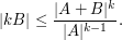
As a corollary, we see that stays quite close to  :
:
But because of the formula (11) and the functional equation, one can in fact deduce the Riemann hypothesis from the apparently weaker statement
where the implied constants can depend on the curve , the prime , and the genus  , but must be independent of the "dimension" . Indeed, from (13) and (12) one can see that the largest magnitude of the (which can be viewed as a sort of "spectral radius" for an underlying operator) is at most ; combining this with the functional equation, one obtains the Riemann hypothesis.
[This is of course only a small part of the story; the proof of (13) is by far the hardest part of the whole proof, and beyond the scope of this article.]
Further reading
The blog post "Amplification, arbitrage, and the tensor power trick" discusses the tensor product trick as an example of a more general "amplification trick".
Comments
Minor correction to 'The tensor power trick'
Tue, 28/07/2009 - 02:31 — Anonymous (not verified)Before (1), the equation for the Fourier transform has \chi when it should have \xi.
Thanks!
Mon, 03/08/2009 - 22:05 — taoFor consistency I've now decided to use \chi throughout that section.
Examples in complexity theory
Tue, 20/12/2011 - 22:54 — g__1. (Approximate counting of problems in
  )
)
Let be the number of satisfying assignments of a Boolean formula
  . Using the leftover hash lemma, there exists a polynomial time probabilistic algorithm taking oracle for SAT that given a formula
  outputs with high probability a number
  such that
i.e. approximates within factor of 2.
By replacing with "tensor power"
  , the number of assignments rises to
  . Running the algorithm on this formula,
and putting we get approximation within factor of
  in time polynomial in
  and length of
  . The algorithm is by Stockmeyer.
2. (Independent set cannot be approximated to a constant factor)
For any constant ,
,  -approximating maximal independent set in a graph is
  -hard. (Taking complement, the same argument goes to clique)
Proof idea:
The PCP theorem implies that there is a constant such that MAX-3SAT cannot be approximated within
  . The usual reduction from 3SAT to independent set takes a formula with
  clauses and gives a graph with
  vertices, where each vertex corresponds to one of 7 ways a clause can be satisfied, and edges correspond to conflicts. Therefore the approximation ratio is preserved, and independent set cannot be approximated within some constant factor. Applying "tensor square"
  allows to lower the constant arbitrarily.
Post new comment
(Note: commenting is not possible on this snapshot.)