How to use the method of stationary phase to control oscillatory integrals

Quick description

The method of stationary phase is a collection of techniques used to estimate oscillatory integrals such as

$\int_{\R^n} a(x) e^{i \lambda \phi(x)}\ dx$

where $a$ is a smooth bump function, $\phi$ is a smooth real-valued phase function, and $\lambda$ is a large real parameter. In many cases (particularly if the stationary points of the phase $\phi$ are isolated and non-degenerate), the methods give not only upper bounds, but a full asymptotic expansion of such integrals.

There are three main pillars of the theory:

Localization (the principle of non-stationary phase) If $\phi$ is non-stationary (i.e. $\nabla \phi \neq 0$ ) on the support of $a$ , then the integral decays very rapidly in $\lambda$ (faster than any power of $\lambda$ ). This is proven by repeated integration by parts or by linearizing the phase. As a consequence, oscillatory integrals can often be localised to individual stationary points, particularly if such points are isolated.

Scaling The magnitude of an oscillatory integral around a stationary point decays at a rate determined by the order of stationarity (or more precisely, on the Newton polytope of the phase at a stationary point). One manifestation of this is the van der Corput lemma for oscillatory integrals.

Asymptotics If the phase is stationary and non-degenerate at a point, then one can perform a change of variables (using Morse theory) to place the phase in a canonical form, e.g. a diagonal quadratic form. This allows one to create asymptotic expansions for the integral around each such stationary point.

If all one is seeking is upper bounds on an integral such as $\int a(x) e^{i\lambda \phi(x)}\ dx$ , and one is fortunate enough to have only one stationary point $x_0$ (i.e. only one solution to the equation $\nabla \phi(x_0) = 0$ , then a "quick and dirty" heuristic for "right" upper bound for this integral is this: the integral should be bounded by the amplitude $|a(x_0)|$ at the stationary point $x_0$ , times the volume of the region $\lambda \phi(x) = \lambda \phi(x_0) + O(1) \}$ near the point of stationary phase where the phase does not oscillate. (This can be viewed as a non-rigorous, oscillatory version of the base times height heuristic.)

Prerequisites

Harmonic analysis

Example 1

Problem (Fresnel-type integral) Let $a \in C^\infty_c(\R)$ be a compactly supported bump function that is non-vanishing at the origin. Obtain as good an upper bound as one can on the magnitude of the integral $= \int_\R e^{i \lambda x^2} a(x)\ dx$ as a function of $\lambda > 0$ . [For sake of discussion, let's not keep track of the dependence on $a$ .]

Solution The base times height bound gives a crude upper bound of $O(1)$ . When $\lambda = O(1)$ , the phase $e^{i\lambda x^2}$ only undergoes a bounded number of oscillations across the compact support of $a$ , so one does not expect any significant improvement to this $O(1)$ bound except when $\lambda$ is large. So now we will assume that $\lambda \gg 1$ .

The phase $\phi(x) = \lambda x^2$ is stationary at $x=0$ . Starting at this stationary point and then moving $x$ away from this point, we see that $\phi$ reaches its first full oscillation (i.e. $\phi(x)=+2\pi$ or $\phi(x)=-2\pi$ ) when $x$ is comparable to $\lambda^{-1/2}$ . After that, it oscillates more and more rapidly, with the wavelengths becoming significantly smaller than $\lambda^{-1/2}$ as one moves away from the origin. So the "base" of this oscillatory integral is of size about $O(\lambda^{-1/2})$ , while the "height" is $O(1)$ , leading to a prediction of $O(\lambda^{-1/2})$ .

To make this argument more precise, what one can do is perform a smooth dyadic partition of unity to decompose the bump function $a$ to a bump function $a_0$ supported on the region $|x| = O(\lambda^{-1/2}) \}$ , plus a telescoping sum of bump functions $a_m$ supported on the dyadic annuli $|x| \sim 2^m \lambda^{-1/2} \}$ , where $2^m$ ranges between $1$ and $O(\lambda^{1/2})$ .

Let's first consider the main term $\int e^{i \lambda x^2} a_0(x)\ dx$ . Here, there is no significant oscillation and one should apply the base times height bound, which gives a contribution of $O(\lambda^{-1/2})$ for this term.

Now let's look at one of the auxiliary terms 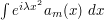$\int e^{i \lambda x^2} a_m(x)\ dx$ . On the region of integration $|x| \sim 2^m \lambda^{-1/2}$ , the phase $\phi(x) = \lambda x^2$ is oscillating at a rate $\phi'(x) = 2 \lambda x$ , which is about $2^m \lambda^{1/2}$ in magnitude; in other words, the phase has a wavelength of about $2^{-m} \lambda^{-1/2}$ . In contrast, the width of the cutoff function $a_m(x)$ is about $2^m \lambda^{-1/2}$ . Since the phase is oscillating faster than the cutoff, there is an opportunity to use integration by parts to exploit cancellation. Indeed, if we write this expression as

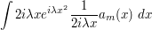
$\int 2 i \lambda x e^{i \lambda x^2} \frac{1}{2 i \lambda x} a_m(x)\ dx$

and integrate by parts, one obtains

$- \int e^{i \lambda x} \frac{d}{dx} [ \frac{1}{2 i \lambda x} a_m(x) ]\ dx.$

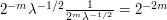Computing the derivative $\frac{d}{dx} [ \frac{1}{2 i \lambda x} a_m(x) ]$ , one sees that the dominant term is $\frac{1}{2i \lambda x} a'_m(x)$ , which has size about $2^{-m} \lambda^{-1/2} \frac{1}{2^m \lambda^{-1/2}} = 2^{-2m}$ . Applying the base times height bound, we thus see that this integral has a size of about $O( 2^{-2m} 2^m \lambda^{-1/2} ) = O( 2^{-m} \lambda^{-1/2} )$ . (Actually, one could repeatedly integrate by parts here and get even better decay in $m$ , but this is already enough decay to sum the series.) Summing in $m$ , one obtains the desired bound of $O( \lambda^{-1/2} )$ for $I(\lambda)$ .

The same analysis shows that if the amplitude function $a$ vanishes to some order $k$ at the origin, then one obtains a bound of $O( \lambda^{-(k+1)/2} )$ for the integral $I(\lambda)$ . The same is true if we take $a$ to be a Schwartz function rather than a bump function. Thus, to obtain asymptotics for $I(\lambda)$ (not just upper bounds), up to an error of $O( \lambda^{-(k+1)/2} )$ , one can replace $a$ with some concrete Schwartz function approximant which agrees with $a$ to $k^{th}$ order at the origin, e.g. a polynomial times the gaussian $e^{-\pi x^2}$ . If one does this, one can get a full asymptotic expansion for $I(\lambda)$ ; see "linearize the phase" for the derivation of the first term of this expansion.

Example 2

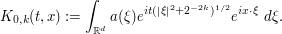
Problem: (Frequency-localized fundamental solution for the Schrodinger equation) Obtain as good a bound as one can for the magnitude of the expression $= \int_{\R^d} a(\xi/2^k) e^{i t |\xi|^2} e^{i x \cdot \xi}\ d\xi$ , where $k$ is an integer, $t \in \R$ , $x \in \R^d$ , and $a$ is a bump function supported on the annulus $1/2 \leq |\xi| \leq 2 \}$ . [For sake of discussion, let's not keep track of the dependence of constants on $d$ and $a$ ; the goal is to get the optimal dependence on $k, t, x$ .]

Solution: Firstly, we normalize parameters by performing the change of variables $\xi = 2^k \eta$ , giving

$K_k(t,x) = 2^{kd} K_0(2^{2k} t, 2^k x ).$

Thus, it suffices to handle the case $k=0$ , as we can then get bounds for the other $k$ by substitution. We are now trying to bound

$K_0(t,x) = \int_{\R^d} a(\xi) e^{i \phi(\xi)}\ d\xi$

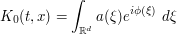
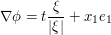
where $\phi$ is the phase

$= t |\xi|^2 + x \cdot \xi.$

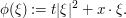
The base times height bound gives an upper bound of $O(1)$ . To do better, we look at the gradient of the phase:

$\nabla \phi(\xi) = 2 t \xi + x.$

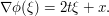
Thus we see that we have just one stationary point, at $-x/2t$ , except when $t$ degenerates to zero.

Let's deal with the degenerate case first. When $t=0$ , we just have a Fourier integral of a bump function; in addition to the trivial bound of $O(1)$ , we will have a bound of $O_N(|x|^{-N})$ for any $N$ by repeated integration by parts, so the correct bound here is $O_N( \langle x \rangle^{-N} )$ (where we write $= (1+|x|^2)^{1/2}$ ). A similar argument also handles the case when $t = O(1)$ ; indeed, in such cases we can simply absorb the $e^{i t |\xi|^2}$ phase into the bump function $\phi(\xi)$ and still get a bump function.

Now let's look at the non-degenerate case, when $|t| \gg 1$ . If $|x|$ is much larger than $|t|$ , e.g. $|x| \geq 10 |t|$ , then the gradient of the phase is always at least $c|x|$ for some absolute constant $c$ , so by repeated integration by parts we see that we can get a bound of $O_N(|x|^{-N})$ in this case. Similarly, if $x$ is much smaller than $t$ , e.g. $|x| \leq |t|/10$ , then the gradient of the phase is always at least $c|t|$ , so by repeated integration by parts we can get a bound of $O_N(|t|^{-N})$ in this case.

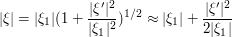
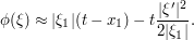
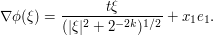
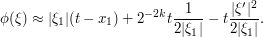
The remaining case is when $|t| \gg 1$ and $|x| \sim |t|$ . Here, we expect the stationary point to lie inside the support of $a$ and so we longer get arbitrary amounts of decay. But we can now use stationary phase. First let's work heuristically: at the stationary point $= -x/2t$ , we have $\nabla^2 \phi = 2t$ , so we can Taylor expand 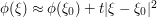$\phi(\xi) \approx \phi(\xi_0) + t |\xi - \xi_0|^2$ . (In fact, this expansion happens to be exact in this case - by completing the square - but we will not exploit this.) Thus, we see that the stationary region $\phi(\xi) = \phi(\xi_0) + O(1)$ consists of those $\xi$ for which $t |\xi-\xi_0|^2 = O(1)$ , which is a ball of radius $O(1/\sqrt{t})$ centred at $\xi_0$ . This ball has volume $O( t^{-d/2} )$ , and the amplitude function $a(x)$ has height $O(1)$ , so by base times height we expect a bound here of $O(t^{-d/2})$ .

One can justify this heuristic by off-the-shelf stationary phase estimates. For instance, one can rewrite the integral as

$\int_{\R^d} a(\xi) e^{i t [ |\xi|^2 + \frac{x}{t} \cdot \xi ]}\ d\xi$

and apply stationary phase with $t$ being the asymptotic parameter and 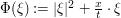$= |\xi|^2 + \frac{x}{t} \cdot \xi$ being the phase; since we are restricting to the region $|x| \sim |t|$ , the phase is uniformly smooth and so the constants arising from the stationary phase bounds will not have any further dependence on $t$ .

Putting everything together, we obtain the following bounds on $|K_k(t,x)|$ , which turn out to be basically optimal:

A bound of $O( t^{-d/2} )$ when $|t| \gg 2^{-2k}$ and $|x| \sim 2^k |t|$ ;
A bound of $O_N( 2^{dk} \langle 1 + 2^{2k} t + 2^{k} x \rangle^{-N} )$ for any $N$ otherwise.

With more work, one can get asymptotics for these integrals, not just upper bounds.

Example 3

Problem: (Frequency-localized fundamental solution for the wave equation) Obtain as good a bound as one can for the magnitude of the expression $= \int_{\R^d} a(\xi/2^k) e^{i t |\xi|} e^{i x \cdot \xi}\ d\xi$ , where $k$ is an integer, $t \in \R$ , $x \in \R^d$ , and $a$ is a bump function supported on the annulus $1/2 \leq |\xi| \leq 2 \}$ .

Solution: Again we can rescale $k=0$ ; this time, the scaling relation is given as

$K_k(t,x) = 2^{kd} K_0(2^{k} t, 2^k x ).$

It is also convenient to exploit some more symmetries: we can flip $(t,x)$ to $(-t,-x)$ at the expense of conjugating $K$ , so can normalize $t \geq 0$ ; similarly, the integral is unchanged under rotation of $x$ , so we may assume $x$ is oriented along the $e_1$ direction, thus $x = x_1 e_1$ for some $x_1 \geq 0$ .

So now we look for upper bounds of $|K_0(t,x)|$ . As before, when $t=O(1)$ we obtain the bounds of $O(1)$ from base times height, and $O_N(|x|^{-N})$ from repeated integration by parts, leading to a net bound of $O_N(\langle x \rangle^{-N})$ in this case.

Now take $t \gg 1$ . Here, the derivative of the phase 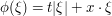$\phi(\xi) = t |\xi| + x \cdot \xi$ is

$\nabla \phi = t \frac{\xi}{|\xi|} + x_1 e_1$ (1)

so a stationary point will now occur along a ray $r > 0 \}$ if $x_1 = t$ , and no stationary point will occur otherwise.

We can dispose of an easy case when $x_1$ is large, e.g. $x_1 \geq 2t$ . Here the phase has gradient at least $cx_1$ everywhere for some $c > 0$ , and repeated integration by parts gives the bound $O_N(x_1^{-N})$ . Similarly, when $x_1$ is small, e.g. $x_1 \leq t/2$ , the gradient is at least $ct$ everywhere, and repeated integration by parts gives the bound $O_N(t^{-N})$ . So we may assume that $t/2 \leq x_1 \leq 2t$ .

We know that the ray $r > 0 \}$ is going to be the most dangerous region, so we now try to localize there. We thus write $\xi = (\xi_1, \xi')$ where $\xi_1 = \xi \cdot e_1$ and $\xi' \in \R^{d-1}$ . In the region where $\xi'$ is large, e.g. $|\xi'| \geq 1/100$ , or when $\xi_1$ is not large and negative, e.g. $\xi_1 \geq -1/4$ , the gradient of the phase $\nabla \phi$ is at least $c t$ by (1), and by smoothly truncating to this portion of the domain of integration we see that the contribution here is $O_N(t^{-N})$ . 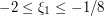So now let us localize to the remaining portion, where $|\xi'| \leq 1/50$ and $-2 \leq \xi_1 \leq -1/8$ , say (the exact numerical values here are not important).

At this point, it can clarify things heuristically to try to linearize the phase. As $\xi_1$ is large and $\xi'$ is small, we can Taylor expand

$|\xi| = |\xi_1| (1 + \frac{|\xi'|^2}{|\xi_1|^2})^{1/2} \approx |\xi_1| + \frac{|\xi'|^2}{2|\xi_1|}$

where we use the approximation $(1+x)^{1/2} \approx 1 + \frac{1}{2} x$ . Thus the phase is roughly of the form

$\phi(\xi) \approx |\xi_1| (t-x_1) - t \frac{|\xi'|^2}{2|\xi_1|}.$

This expansion highlights the fact that the phase $\phi$ is at its most stationary when $\xi' = 0$ and $t=x_1$ .

Let's first handle the extreme case $t=x_1$ . Here, the phase is indeed stationary at $\xi'=0$ (where it is zero), and the stationary region is basically the cylinder where $\xi' = O( t^{-1/2} )$ . This cylinder has volume $O( t^{-(d-1)/2} )$ , so this would heuristically be the bound for the integral in this case. To do this rigorously (and using the original phase, rather than the heuristic approximation to this phase), one can perform (smooth) dyadic decomposition to this cylinder, plus the remaining cylinders $\{ 2^{m-1} t^{-1/2} \leq |\xi'| \leq 2^{m+2} t^{-1/2} \}$ . The original cylinder yields a contribution of $O( t^{-(d-1)/2} )$ by the base times height bound. On the remaining cylinders, there is some non-trivial oscillation in the $|\xi'|$ direction; exploiting that by repeated integration by parts, we eventually see that the contribution of the $m^{th}$ cylinder is 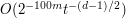$O( 2^{-100m} t^{-(d-1)/2} )$ (say), so on summing we do get $O( t^{-(d-1)/2} )$ as claimed.

Now we can handle the general case $t \neq x_1$ . This is as before, but now there is also some oscillation along the $e_1$ axis as well as in the $\xi'_1$ direction. For instance, in the cylinder 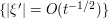$\{ |\xi'| = O( t^{-1/2} ) \}$ , we can improve upon the trivial bound of $O( t^{-(d-1)/2} )$ to o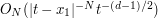btain $O_N( |t-x_1|^{-N} t^{-(d-1)/2} )$ for any $N$ , and similarly for the other cylinders, to on summing we now get a net bound of $O_N( |t-x_1|^{-N} t^{-(d-1)/2} )$ .

Putting all this together, we get the bounds

$K_k(t,x) = O_N( 2^{dk} \langle 2^k (|t| - |x|) \rangle^{-N} \langle 2^k t \rangle^{-(d-1)/2})$

for all $k,t,x$ .

Example 4

Problem: (Frequency-localized fundamental solution for the Klein-Gordon equation) Obtain as good a bound as one can for the magnitude of the expression $= \int_{\R^d} a(\xi/2^k) e^{i t \langle \xi\rangle} e^{i x \cdot \xi}\ d\xi$ , where $k$ is an integer, $t \in \R$ , $x \in \R^d$ , and $a$ is a bump function supported on the annulus $1/2 \leq |\xi| \leq 2 \}$ .

Solution: This is a particularly tricky one, requiring quite a few computations and cases.

Once again, we try to rescale $k=0$ . But this time, we run into a hitch: the phase $\langle \xi \rangle$ is not scale-invariant, so we cannot eliminate $k$ completely. Instead, we get

$K_k(t,x) = 2^{kd} K_{0,k}(2^{k} t, 2^k x )$

where

$= \int_{\R^d} a(\xi) e^{i t (|\xi|^2 + 2^{-2k})^{1/2}} e^{i x \cdot \xi}\ d\xi.$

As before, we can exploit some symmetries and reduce to the case $t \geq 0$ and $x = x_1 e_1$ for some $x_1 > 0$ .

If we first look at the limit $k \to +\infty$ , we see that this integral collapses to the integral considered in the preceding exercise. At the other extreme $k \to -\infty$ , we have a Taylor expansion

$(|\xi|^2 + 2^{-2k})^{1/2} = 2^{-k} (1 + 2^{2k} |\xi|^2)^{1/2} \approx 2^{-k} + \frac{1}{2} 2^k |\xi|^2$ (2)

and the situation begins to more closely resemble the Schrodinger example. So it looks like we may have to divide into cases, with large $k$ behaving like the wave equation, and small $k$ behaving like the Schrodinger equation.

The case $k \leq 0$ can in fact be handled by the Schrodinger methods without much difficulty. Guided by the approximation (2), we can write

$(|\xi|^2 + 2^{-2k})^{1/2} = 2^{-k} + 2^k \phi_k(\xi)$

and one checks that $\phi_k$ is smooth on the support of $a$ uniformly for $k \leq 0$ , and furthermore $\nabla^2 \phi_k$ is uniformly non-degenerate. Off-the-shelf stationary phase tools then give the bound 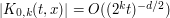$|K_{0,k}(t,x)| = O( (2^k t)^{-d/2} )$ if $2^k t \gg 1$ and $|x| \sim 2^k t$ , and $|K_{0,k}(t,x)| = O_N( \langle |2^k t| + |x|\rangle^{-N} )$ for any $N > 0$ otherwise.

Now let's look at the case when $k \geq 0$ . As before, we get a bound of $O_N( \langle x \rangle^{-N} )$ when $t = O(1)$ , so suppose $t \gg 1$ .

The gradient of the phase $\phi(\xi) = t (|\xi|^2 + 2^{-2k})^{1/2} + x \cdot \xi$ is

$\nabla \phi(\xi) = \frac{t \xi}{(|\xi|^2 + 2^{-2k})^{1/2}} + x_1 e_1.$ (3)

As in the wave case, we can then use repeated integration by parts to obtain a decay of $O_N( \langle x \rangle^{-N} )$ when $x_1 \gg t$ and $O_N( \langle t \rangle^{-N} )$ when $x_1 \ll t$ , so we can restrict attention to the case when $x_1 \sim t$ .

We expect the phase to be stationary near the negative $e_1$ axis, so we try Taylor expansion around that ray. Writing $\xi = (\xi_1,\xi')$ as before, we obtain

$\phi(\xi) \approx |\xi_1| (t-x_1) + 2^{-2k} t \frac{1}{2|\xi_1|} - t \frac{|\xi'|^2}{2|\xi_1|}.$ (4)

In the case when $1 \ll t \ll 2^{2k}$ , the term $2^{-2k} t \frac{1}{2|\xi_1|}$ is of bounded size, and so we do not expect this term to contribute much to the bounds. In other words, in this case the bounds should be the same as those for the wave equation, namely 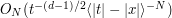$O_N( t^{-(d-1)/2} \langle |t|-|x| \rangle^{-N} )$ for any $N$ . And indeed, one can check that the arguments in the previous exercise can be repeated in this range of $t$ to give the stated bound.

Finally, we look at the case when $t \gg 2^{2k}$ . If $|t-x_1|$ is much larger than $2^{-2k} t$ , then the phase oscillation from the $|\xi_1| (t-x_1)$ term is greater than that from the $2^{-2k} t \frac{1}{2|\xi_1|}$ term, so the wave equation arguments will still give a bound of $O_N( t^{-(d-1)/2} \langle |t|-|x| \rangle^{-N} )$ .

If instead 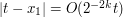$|t-x_1| = O( 2^{-2k} t )$ , then the portion 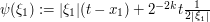$= |\xi_1| (t-x_1) + 2^{-2k} t \frac{1}{2|\xi_1|}$ of the (Taylor approximation of the) phase will have a stationary point, with a second derivative of roughly $2^{-2k} t$ . From the approximation (4), we thus expect the stationary region to have size about $(2^{-2k} t)^{-1/2}$ in the $\xi_1$ direction and $O( t^{-1/2} )$ in the other directions, leading to a prediction of $O( 2^k t^{-d/2} )$ for the size of the integral. This can be made rigorous by first dividing the region of integration into cylinders as in the previous example (i.e. smoothly partitioning the $\xi'$ variable around the critical value $\xi' = 0$ ), and then partitioning those cylinders further in the $\xi_1$ direction, based on the stationary point indicated in (3). We omit the rather tedious computations, and instead just give the final bounds for $K_k(t,x)$ after putting all the above cases together, which are

$|K_{0,k}(t,x)| = O( 2^{kd} (2^{2k} t)^{-d/2} )$ if $k \leq 0$ , $2^{2k} t \gg 1$ and $|x| \sim 2^k t$ ;
$|K_{0,k}(t,x)| = O_N( 2^{kd} \langle |2^{2k} t| + |2^k x|\rangle^{-N} )$ for any $N > 0$ in all other cases with $k \leq 0$ ;
$|K_{0,k}(t,x)| = O_N( 2^{kd} \langle 2^k t\rangle^{-(d-1)/2} \langle 2^k(|t|-|x|) \rangle^{-N} )$ when $k > 0$ and $|t| \leq 2^k$ or $2^k(|t|-|x|) \gg 2^{-k} |t|$ ;
$|K_{0,k}(t,x)| = O_N( 2^{kd} 2^k (2^k t)^{-d/2} )$ if $k \geq 0$ , $|t| > 2^k$ , and $2^k(|t|-|x|) = O(2^{-k} |t|)$ .

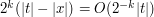General discussion

The methods can be adapted to deal with more general amplitude functions $a(x)$ than bump functions by such tools as (smooth) dyadic decomposition.

A good discussion of the technique can be found in Stein's book on harmonic analysis.

The more classical method of steepest descent, based on contour shifting, can also reproduce some of the results of stationary phase.

A variant of the base times height heuristic can give a means to predict the right order of magnitude of an oscillatory integral $\int_{\R^n} a(x) e^{i\lambda \phi(x)}$ near a stationary point $x_0$ : the magnitude should roughly equal the "height" $|a(x_0)|$ , times the size of the "base", defined as the set of points $x$ near $x_0$ where $\phi(x)$ is within $O(1/\lambda)$ of $\phi(x_0)$ (i.e. the region near the stationary point $x_0$ where phase has not yet begun to oscillate). For instance, $\int_{\R^n} a(x) e^{i\lambda|x|^2}$ should be about $|a(0)| \lambda^{-n/2}$ in magnitude.

Post new comment

(Note: commenting is not possible on this snapshot.)